Decision Tree Challenge 2017-12-05, written by 김대남

#datascience #decisiontree

교과서만 보고 맨땅에 헤딩 해보기

데이터 사이언스 교과서의 Chapter 4. Fitting a Model to Data의 선형 회귀 분석 또는 SVM 등을 해보려 하였으나 여러가지 이유로 Chapter 3. Introduction to Predictive Modeling의 결정 트리 직접 만들기를 맨땅에 헤딩해 보았다. >.< 트리만 하더라도 다양한 알고리즘과 논문들이 존재하지만 개념을 먼저 잡고 가자는 취지로 교과서만을 중심으로 직접 만들어보았다.

엔트로피

엔트로피(Entropy)는 어떤 집합의 무질서 정도를 측정하는 수치이다. 범위는 0부터 1까지로 나타내며 엔트로피가 0이면 완전 순수하며 1이면 완전 불순하다는 것을 의미한다. 다음은 책에서 설명하는 엔트로피의 공식과 그래프이다.

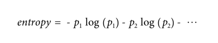
from Data Science for Business, Equation 3-1. Entropy

p는 특정 값의 비율을 나타내며 0.5(50%)가 될 경우 가장 큰 값, 즉 아주 불순하게된다. 아래 그래프를 통해서 +와 -가 같은 비율일 경우가 가장 불순한 상태인 것을 의미한다.

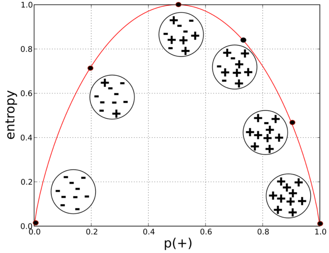
from Data Science for Business, Figure 3-3. Entropy of a two-class set as a function of p(+).

정보 증가량

엔트로피가 데이터의 순수한 정도를 확인하는 작업이라면 정보 증가량(Information Gain, IG)은 우리가 알고자 하는 타겟에 관련해서 어떤 속성(Attribute Segement)이 얼마나 많은 정보를 제공할 수 있는지를 확인하는 과정이다. 이를 위해서 전체 데이터를 각 속성을 기준으로 분할하여 정보 증가량을 계산하며 분할과 계산을 반복적으로 진행하여 각 속성에 대한 엔트로피를 최대한 작은 값으로 만드는 것이다. 거꾸로 말하면 children의 엔트로피가 낮은 것일수록 정보의 증가량이 커진다는 것을 알 수 있다.

그 수식은 아래와 같으며 parent는 아무 속성도 적용하지 않은 전체 데이터에 대한 데이터이다.

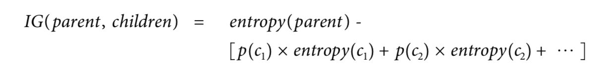
from Data Science for Business, Equation 3-2. Information gain

정보를 전달하는 속성의 선택

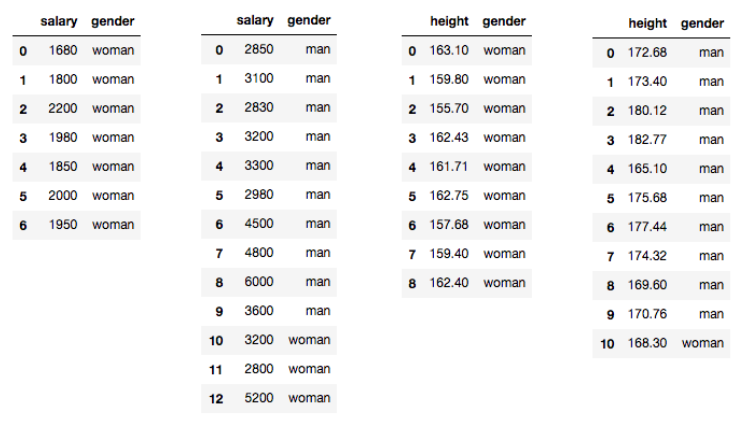
테스트로 간단한 데이터를 임의로 만들어서 확인 해보자. 데이터는 통계청 평균 신장과 e-나라지표의 평균 임금 데이터를 가지고 임의로 작성하였다.

어떤 그룹에 20명이 있는데 그 중에 남자와 여자가 10명씩 있을 경우 gender를 알고 싶다고 가정하자. (여기서는 감독 학습을 사용한다.) gender에 대한 엔트로피는 다음과 같이 Python 코드로 확인할 수 있다.

import math
import pandas as pd

genders = ['man', 'woman']
people = [
    {'gender': 'man', 'salary': 285, 'height': 172.68},
    {'gender': 'man', 'salary': 260, 'height': 173.4},
    {'gender': 'man', 'salary': 283, 'height': 180.12},
    {'gender': 'man', 'salary': 320, 'height': 182.77},
    {'gender': 'man', 'salary': 330, 'height': 165.1},
    {'gender': 'man', 'salary': 298, 'height': 175.68},
    {'gender': 'man', 'salary': 450, 'height': 177.44},
    {'gender': 'man', 'salary': 480, 'height': 174.32},
    {'gender': 'man', 'salary': 600, 'height': 169.6},
    {'gender': 'man', 'salary': 360, 'height': 170.76},
    {'gender': 'woman', 'salary': 168, 'height': 168.1},
    {'gender': 'woman', 'salary': 120, 'height': 159.8},
    {'gender': 'woman', 'salary': 200, 'height': 155.7},
    {'gender': 'woman', 'salary': 210, 'height': 174.3},
    {'gender': 'woman', 'salary': 198, 'height': 172.43},
    {'gender': 'woman', 'salary': 185, 'height': 169.71},
    {'gender': 'woman', 'salary': 280, 'height': 162.75},
    {'gender': 'woman', 'salary': 200, 'height': 157.68},
    {'gender': 'woman', 'salary': 195, 'height': 159.4},
    {'gender': 'woman', 'salary': 310, 'height': 169.4}
]


def get_p(a, b):
    len_a = len(a)
    len_b = len(b)

    if len_a == 0:
        len_a = 0.00000001
    
    if len_b == 0:
        len_b = 0.00000001
        
    return len_a / len_b


def get_entropy_params(labels, data):
    return (
        get_p(data[data['gender'] == labels[0]], data),
        get_p(data[data['gender'] == labels[1]], data)
    )


def get_entropy(labels, data):
    ps = get_entropy_params(labels, data)
    return -sum([p * math.log(p, 2) for p in ps])


data = pd.DataFrame(people)
print('Entropy is ' + str(get_entropy(genders, data)))

# [output]
# Entropy is 1.0

gender 에 대해서만 엔트로피를 확인 했을 경우 엔트로피는 1이며 매우 불순한 데이터라고 보여진다. 그러나 각 속성을 이용해서 gender에 대한 엔트로피를 계산할 경우 다음과 같이 확인할 수 있다.

위 표를 보면 가장 왼쪽 부터 순서대로 임금이 230만원 보다 작은 경우와 크거나 같은 경우, 신장이 164센티미터 보다 작은 경우와 크거나 같은 경우로 분류된 값이다. 한 눈에 보아도 데이터의 순도가 좋아졌음을 알 수 있다.

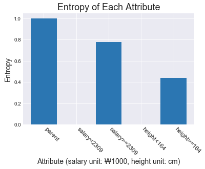
속성별 엔트로피를 그래프로 확인하면 아무 속성도 적용하지 않은 전체 데이터의 경우(parent) 엔트로피가 가장 좋지 못하며 임금이 230만원 보다 작을 경우와 신장이 164센티미터 보다 작을 경우 엔트로피가 0(실제로는 매우 작은 수) 임을 확인할 수 있다.

신장을 이용해서 분류할 경우 정보의 증가량이 가장 높음을 알 수 있으며 이를 이용해서 분할한 데이터에 다시 한 번 정보 증가량을 계산하고 정보의 증가량이 가장 높은 속성으로 반복적으로 분할하는 방법을 사용한다.

엔트로피와 정보의 증가량을 이용해서 데이터를 분류하는 이유는 결국에 우리가 알고자 하는 gender를 가장 잘 예측할 수 있는 모델을 만들기 위함이다.

결정 트리 작성 및 테스트

이번에는 교과서에서 다루는 대손 상각 예시의 데이터를 적절히 조합해서 실제 트리를 만들고 테스트를 해보도록 하자. 이 때, 테스트는 학습용으로 만든 데이터를 그대로 사용할 것이기 때문에 정확도가 다소 높을 수 있으나 무시하도록 하자. 이 포스트에서는 결정 트리를 스크래치 코드로 만들어서 동작시켜 보는 것이 목표이기 때문이다.

트리 생성 로직을 아래와 같이 작성했다. 로직의 핵심은 정보의 증가량을 기반으로 분할 정복을 반복해서 실행하도록 하는 것이다.

def create_tree(tree, labels, attributes, inputs, depth=0, max_depth=10, node_id=None, direction=None):
    if tree is None:
        return

    """
    Conditions to become a terminal node.
    
    1. At the entropy is smaller than "entropy_limit".
    2. At no left or right data after dividing by the "attribute".
    3. At the specific "max_depth".
    """
    igs, entropies = get_information_gain(labels, attributes , inputs)
    igs_sorted  = sorted(igs.items(), key=lambda x: x[1], reverse=True)
    igs_max = igs_sorted[0]
    attr_key = igs_max[0]
    attr_values = attributes[attr_key]
    mode = attr_values[0]
    if mode == 'int':
        v = attr_values[1]
        inputs_left = inputs[inputs[attr_key] < v]
        inputs_right = inputs[inputs[attr_key] >= v]
    else:
        inputs_left = inputs[inputs[attr_key] == attr_values[1]]
        inputs_right = inputs[inputs[attr_key] == attr_values[2]]

    inputs_left.reset_index(inplace=True)
    inputs_right.reset_index(inplace=True)
    del inputs_left['index']
    del inputs_right['index']
    if node_id is None:
        node_id = 1

    node_data = {
        'id': node_id,
        'key': attr_key,
        'values': attr_values[1:],
        'mode': mode,
        'depth': depth,
        'direction': direction,
    }

    entropy_limit = 0.1
    
    if (depth >= max_depth) or len(inputs_left) == 0 or len(inputs_right) == 0 or \
        get_entropy(labels, inputs_left) < entropy_limit or get_entropy(labels, inputs_right) < entropy_limit:

        next_node = tree.add(**node_data)
        next_node.update(**get_terminal_node_data(node_id, depth, direction, labels, inputs))
        return
    elif depth == 0:
        next_node = tree.update(**node_data)
    else:
        next_node = tree.add(**node_data)

    if depth == 0:
        # Update attributes based on the biggest IG at the first time only.
        next_attributes = {k: v for k, v in attributes.items() if k != attr_key}
    else:
        next_attributes = attributes
    
    create_tree(next_node, labels, next_attributes, inputs_left, depth + 1, max_depth, node_id * 2, 'left')
    create_tree(next_node, labels, next_attributes, inputs_right, depth + 1, max_depth, (node_id * 2) + 1, 'right')
        
tree = Tree()
# Remove "residence" attribute because its IG is lower than others.
create_tree(tree, LABELS, {k: v for k, v in ATTRIBUTES.items() if k != 'residence'}, INPUTS)
tree.__str__()

실행 결과 다음과 같은 트리 데이터가 나왔다.

{'id': 4, 'key': None, 'values': None, 'mode': None, 'depth': 2, 'direction': 'left', 'evaluation': 'WRITE-OFF'}
{'id': 2, 'key': 'balance', 'values': [50000000], 'mode': 'int', 'depth': 1, 'direction': 'left', 'evaluation': None}
{'id': 5, 'key': None, 'values': None, 'mode': None, 'depth': 2, 'direction': 'right', 'evaluation': 'NO-WRITE-OFF'}
{'id': 1, 'key': 'employed', 'values': ['True', 'False'], 'mode': 'str', 'depth': 0, 'direction': None, 'evaluation': None}
{'id': 3, 'key': None, 'values': None, 'mode': None, 'depth': 1, 'direction': 'right', 'evaluation': 'WRITE-OFF'}

그래프를 그려보면 다음과 같다.

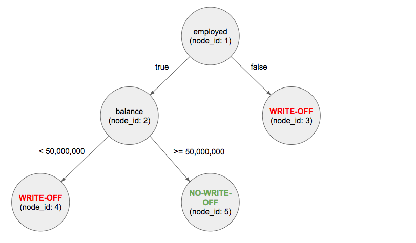
그래프를 보고 잠시 생각을 해보면 대손 상각이 발생할 조건과 정상 상환 할 조건은 다음과 같다.

• 대손 상각: 직업이 없거나 직업이 있어도 통장 잔액이 5천만원 미만인 경우.
• 정상 상환: 직업이 있고 통잔 잔액이 5천만원 이상인 경우.

그럼 이제 데이터를 넣고 테스트를 해보자.

inputs = list(INPUTS.T.to_dict().values())
for data in inputs:
    data['evaluation'] = tree.evaluate(**data)

evaluations = pd.DataFrame(inputs)
evaluations = evaluations[['age', 'balance', 'employed', 'residence', 'label', 'evaluation']]
display(evaluations)

no_write_off = evaluations[(evaluations['label'] == True) & (evaluations['evaluation'] == 'NO-WRITE-OFF')]
write_off = evaluations[(evaluations['label'] == False) & (evaluations['evaluation'] == 'WRITE-OFF')]
total = len(evaluations)
matched = len(no_write_off) + len(write_off)
print('Accuracy is ' + str(matched / total))

# [output]
# Accuracy is 0.9

무려 90%의 정확도를 나타낸다!!! 여기서 끝이 아니다. 실제로는 매우 다양한 속성에 대한 전처리, 인사이트 분석, 확률 분석, 초평면에 대한 이해 등 다룰 것이 많으나 차근 차근 하나씩 익혀 나가도록 하자.
다음에는 선형 회귀 분석에 대해서 코드를 직접 만들어보도록 하겠다.

참고

• 자작 결정 트리
• 데이터 사이언스 교과서

#datascience #decisiontree